3. Introduction to spatial data in R
Foreword on working directory, data and packages
The Data for this tutorial are provided via Github. In order to reproudce the code with your own data, replace the url with your local filepath
If you work locally, you may define the working directory
setwd("YOUR/FILEPATH")
# this will not work. if you want to use it, define a path on your computer
This should be the place where your data and other folders are stored. more Information can be found here
Code chunks for saving data and results are disabeled in this tutorial (using a #). Please replace (“YOUR/FILEPATH”) with your own path.
The code is written in such a way, that packages will be automatically installed (if not already installed) and loaded. Packages will be stored in the default location of your computer.
Intro
The sp package (spatial) provoides Classes and methods for spatial (vector) data; the classes document where the spatial location information resides, for 2D or 3D data. Utility functions are provided, e.g. for plotting data as maps, spatial selection, as well as methods for retrieving coordinates, for subsetting, print, summary, etc.
The sf package (simple features = points, lines, polygons and their respective ‘multi’ versions) is the new kid on the block with further functions to work with simple features, a standardized way to encode spatial vector data. It binds to the packages ‘GDAL’ for reading and writing data, to ‘GEOS’ for geometrical operations, and to ‘PROJ’ for projection conversions and datum transformations.
For the time being, it is best to know and use both the sp and the sf packages, as discussed in this post. However, we focus on the sf package. for the following reasons:
- sf ensures fast reading and writing of data
- sf provides enhanced plotting performance
- sf objects can be treated as data frames in most operations
- sf functions can be combined using
%>%operator and works well with the tidyverse collection of R packages. - sf function names are relatively consistent and intuitive (all begin with
st_)
However, in some cases we need to transform sf objects to sp objects or vive versa. In that case, a simple transformation to the desired class is necessary:
To sp object <- as(object, Class = "Spatial")
To sf object_sf = st_as_sf(object_sp, "sf")
A word of advice: be flexible in the usage of sf and sp. Sometimes it may be hard to explain why functions work for one data type and do not for the other. But since transformation is quite easy, time is better spend on analyzing your data than on wondering why operations do not work.
Apply a free interpretation of Paul Feyerabend’s “anything goes” argument and use sf and sp packages as you like - and as they work for you.
Now we will begin by exploring simple features.
Load the required sf and sp packages. Packages can be loaded with the library() function in R.
if (!require(sp)){install.packages("sp"); library(sp)}
if (!require(sf)){install.packages("sf"); library(sf)}
Treating spatial data like data frames and ploting them
Most of the time, we already have spatial data and want to explore them. With the sf package, this can be done similarily to data frames with base R.
First we will use the world dataset provided by the spData. spData offers a large variety of spatial datasets for demonstrating, benchmarking and teaching spatial data analysis. It includes R data of class sf (defined by the package ‘sf’), Spatial (‘sp’), and nb (‘spdep’). Unlike other spatial data packages such as ‘rnaturalearth’ and ‘maps’, it also contains data stored in a range of file formats including GeoJSON, ESRI Shapefile and GeoPackage. Some of the datasets are designed to illustrate specific analysis techniques. cycle_hire() and cycle_hire_osm(), for example, is designed to illustrate point pattern analysis techniques. To see all available data sets use ls("package:spData").
# load spData to get the data set
if (!require(spData)){install.packages("spData"); library(spData)}
if (!require(lwgeom)){install.packages("lwgeom"); library(lwgeom)}
We can now perform exploratory operations with this sf object as we did with a regular data frame:
names(world)## [1] "iso_a2" "name_long" "continent" "region_un" "subregion" "type"
## [7] "area_km2" "pop" "lifeExp" "gdpPercap" "geom"plot(world)## Warning: plotting the first 9 out of 10 attributes; use max.plot = 10 to plot
## all
world[1:10,2] # first 10 rows of 2. column## Simple feature collection with 10 features and 1 field
## Geometry type: MULTIPOLYGON
## Dimension: XY
## Bounding box: xmin: -180 ymin: -55.25 xmax: 180 ymax: 83.23324
## Geodetic CRS: WGS 84
## # A tibble: 10 x 2
## name_long geom
## <chr> <MULTIPOLYGON [°]>
## 1 Fiji (((-180 -16.55522, -179.9174 -16.50178, -179.7933 -16.02088~
## 2 Tanzania (((33.90371 -0.95, 31.86617 -1.02736, 30.76986 -1.01455, 30~
## 3 Western Sahara (((-8.66559 27.65643, -8.817828 27.65643, -8.794884 27.1207~
## 4 Canada (((-132.71 54.04001, -133.18 54.16998, -133.2397 53.85108, ~
## 5 United States (((-171.7317 63.78252, -171.7911 63.40585, -171.5531 63.317~
## 6 Kazakhstan (((87.35997 49.21498, 86.82936 49.82667, 85.54127 49.69286,~
## 7 Uzbekistan (((55.96819 41.30864, 57.09639 41.32231, 56.93222 41.82603,~
## 8 Papua New Guinea (((141.0002 -2.600151, 141.0171 -5.859022, 141.0339 -9.1178~
## 9 Indonesia (((104.37 -1.084843, 104.0108 -1.059212, 103.4376 -0.711945~
## 10 Argentina (((-68.63401 -52.63637, -68.63335 -54.8695, -67.56244 -54.8~# summrizing statistics and indexing/subsetting to the attribute (collumn) lifExp
summary(world["lifeExp"])## lifeExp geom
## Min. :50.62 MULTIPOLYGON :177
## 1st Qu.:64.96 epsg:4326 : 0
## Median :72.87 +proj=long...: 0
## Mean :70.85
## 3rd Qu.:76.78
## Max. :83.59
## NA's :10#more subestting
plot(world[3:6])
plot(world["pop"])
# isolate asia and then plot it
world_asia <- world[world$continent == "Asia", ]
plot(world_asia)
## Warning: plotting the first 9 out of 10 attributes; use max.plot = 10 to plot
## all For more advanced map making, dedicated visualization packages such as tmap are recommended. We will do that at a later stage. For now it is sufficient to know that basic map visualizations are possible with the sf package.
Understanding sf objects
Simple features, in the most basic definition, consist of spatial and non-spatial attributes.
class(world)## [1] "sf" "tbl_df" "tbl" "data.frame"Lets take a look at the the object:
world[1:10, ]## Simple feature collection with 10 features and 10 fields
## Geometry type: MULTIPOLYGON
## Dimension: XY
## Bounding box: xmin: -180 ymin: -55.25 xmax: 180 ymax: 83.23324
## Geodetic CRS: WGS 84
## # A tibble: 10 x 11
## iso_a2 name_l~1 conti~2 regio~3 subre~4 type area_~5 pop lifeExp gdpPe~6
## <chr> <chr> <chr> <chr> <chr> <chr> <dbl> <dbl> <dbl> <dbl>
## 1 FJ Fiji Oceania Oceania Melane~ Sove~ 1.93e4 8.86e5 70.0 8222.
## 2 TZ Tanzania Africa Africa Easter~ Sove~ 9.33e5 5.22e7 64.2 2402.
## 3 EH Western~ Africa Africa Northe~ Inde~ 9.63e4 NA NA NA
## 4 CA Canada North ~ Americ~ Northe~ Sove~ 1.00e7 3.55e7 82.0 43079.
## 5 US United ~ North ~ Americ~ Northe~ Coun~ 9.51e6 3.19e8 78.8 51922.
## 6 KZ Kazakhs~ Asia Asia Centra~ Sove~ 2.73e6 1.73e7 71.6 23587.
## 7 UZ Uzbekis~ Asia Asia Centra~ Sove~ 4.61e5 3.08e7 71.0 5371.
## 8 PG Papua N~ Oceania Oceania Melane~ Sove~ 4.65e5 7.76e6 65.2 3709.
## 9 ID Indones~ Asia Asia South-~ Sove~ 1.82e6 2.55e8 68.9 10003.
## 10 AR Argenti~ South ~ Americ~ South ~ Sove~ 2.78e6 4.30e7 76.3 18798.
## # ... with 1 more variable: geom <MULTIPOLYGON [°]>, and abbreviated variable
## # names 1: name_long, 2: continent, 3: region_un, 4: subregion, 5: area_km2,
## # 6: gdpPercapThe summary above gives us a lot of information on the Simple feature. On the non-spatial side, we can see that it has 177 features and 10 fields. Let’s think of it as a usual spreadsheet or, to stay in GIS terms, an attribute table.
On the spatial side, we get information on geographical data e.g. the “real world”. Namely the fields geometry type, dimension, bbox and CRS information - epsg (SRID) and proj4string. They are briefly introduced:
Geometry types
Der Punkt als Träger der geometrischen Information
All geometries boil down to one or more points. The most common geometry types are points, lines, polygons and their respective ‘multi’ versions.
The geometry type of the world object is Multipolygon.
Dimension
Refers to the dimension the data is displayed. Cartesian coordinate system in eiter two (XY) or or thre dimensions (XYZ or rarely XYM).
Bounding box (bbox)
The bounding box is the minimum or smallest bounding or enclosing box of a point, line or polygon or their respective ‘multi’ versions. It defines the extent of a geometry in xmin, ymin, xmax and ymax; depending on the coordinate reference system, the values of the bbox are either spherical (lon/lat) or projected e.g. cartesian coordinates.
# Load the rmarkdown package in order to load figure
if (!require(rmarkdown)){install.packages("rmarkdown"); library(rmarkdown)}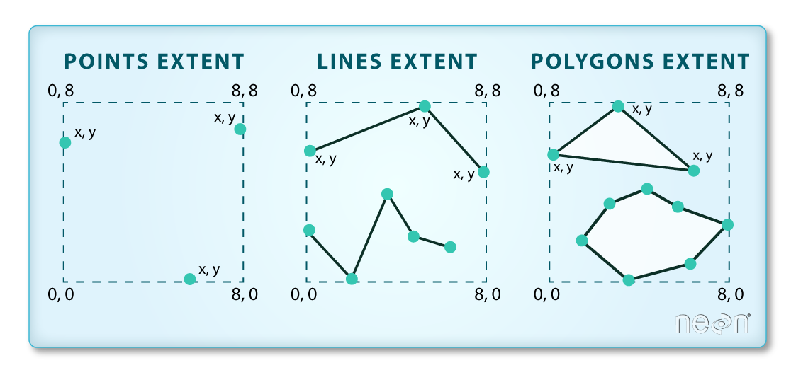
Examples of bounding boxes for different geometries
The bounding box of an object can be retrieved separately:
st_bbox(world)## xmin ymin xmax ymax
## -180.00000 -89.90000 179.99999 83.64513Coordinate reference systems (crs)
In geography, a coordinate system is a reference system that enables every location on Earth to be specified by a set of numbers, letters or symbols. Each CRS is defined by:
- Its measurement framework, which is either geographic (in which spherical coordinates are measured from the earth’s center) or projected e.g. planimetric (in which the earth’s coordinates are projected onto a two-dimensional planar surface)
- Its units of measurement (feet/meters for projected, lon/lat degrees for geographic)
- For projected coordinate systems a definition of the map projection
- Other measurement system properties such as a spheroid of reference, a datum, one or more standard parallels, a central meridian, and possible shifts in the x- and y-directions
A brief summary of what coordinate systems are is given here.
In R, there are two ways to describe a crs. Either by using the epsg code or the proj4string definition.
EPSG (SRID)
The European Petroleum Survey Group Geodesy (EPSG) is best known for its system of spatial reference IDs for coordinate systems. An EPSG code is aunique ID that can be a simple way to identify a CRS.
Use st_crs to extract coordinate system (CS) information from an sf object. This gives us the EPSG code and the PROJ4 projection string.
st_crs(world)## Coordinate Reference System:
## User input: EPSG:4326
## wkt:
## GEOGCRS["WGS 84",
## DATUM["World Geodetic System 1984",
## ELLIPSOID["WGS 84",6378137,298.257223563,
## LENGTHUNIT["metre",1]]],
## PRIMEM["Greenwich",0,
## ANGLEUNIT["degree",0.0174532925199433]],
## CS[ellipsoidal,2],
## AXIS["geodetic latitude (Lat)",north,
## ORDER[1],
## ANGLEUNIT["degree",0.0174532925199433]],
## AXIS["geodetic longitude (Lon)",east,
## ORDER[2],
## ANGLEUNIT["degree",0.0174532925199433]],
## USAGE[
## SCOPE["Horizontal component of 3D system."],
## AREA["World."],
## BBOX[-90,-180,90,180]],
## ID["EPSG",4326]]A list of epsg codes can be found here.
The EPSG code may not always be available for a particular coordinate system, but if a spatial object has a defined coordinate system, it will always have a PROJ4 projection string. Its multi-parameter syntax is briefly discussed next.
proj4string
PROJ is a generic coordinate transformation software that transforms geospatial coordinates from one coordinate reference system (CRS) to another. The PROJ4 syntax consists of a list of parameters used in defining a coordinate system. The parameters are combined in a single string by the + character. Most common parameters are:
| Parameter | Description |
|---|---|
| +proj | Projection name |
| +ellps | Ellipsoid name |
| +datum | Datum name |
| +units | meters, US survey feet, etc. |
| +x_0 | False easting |
| +lat_0 | Latitude of origin |
Further information can be found on the PROJ4 website. If you know the SRID of your crs, you can copy the PROJ4 syntax from this website.
Assigning and transforming crs
Assigning and transformation the crs of an sf object is relatively straight forward. We subset the world data to Canada.
canada <- world[world$name_long == "Canada", ]In cases when a coordinate reference system (CRS) is missing or the wrong CRS is set, the st_set_crs() function can be used. st_transform will convert to a different crs. All these functions are demonstrated below with the canada object.
st_crs(canada)## Coordinate Reference System:
## User input: EPSG:4326
## wkt:
## GEOGCRS["WGS 84",
## DATUM["World Geodetic System 1984",
## ELLIPSOID["WGS 84",6378137,298.257223563,
## LENGTHUNIT["metre",1]]],
## PRIMEM["Greenwich",0,
## ANGLEUNIT["degree",0.0174532925199433]],
## CS[ellipsoidal,2],
## AXIS["geodetic latitude (Lat)",north,
## ORDER[1],
## ANGLEUNIT["degree",0.0174532925199433]],
## AXIS["geodetic longitude (Lon)",east,
## ORDER[2],
## ANGLEUNIT["degree",0.0174532925199433]],
## USAGE[
## SCOPE["Horizontal component of 3D system."],
## AREA["World."],
## BBOX[-90,-180,90,180]],
## ID["EPSG",4326]]# set crs to NA
st_crs(canada) <- NA
st_crs(canada)## Coordinate Reference System: NA# assign crs back with epsg code
st_crs(canada) <- 4326
st_crs(canada)## Coordinate Reference System:
## User input: EPSG:4326
## wkt:
## GEOGCRS["WGS 84",
## DATUM["World Geodetic System 1984",
## ELLIPSOID["WGS 84",6378137,298.257223563,
## LENGTHUNIT["metre",1]]],
## PRIMEM["Greenwich",0,
## ANGLEUNIT["degree",0.0174532925199433]],
## CS[ellipsoidal,2],
## AXIS["geodetic latitude (Lat)",north,
## ORDER[1],
## ANGLEUNIT["degree",0.0174532925199433]],
## AXIS["geodetic longitude (Lon)",east,
## ORDER[2],
## ANGLEUNIT["degree",0.0174532925199433]],
## USAGE[
## SCOPE["Horizontal component of 3D system."],
## AREA["World."],
## BBOX[-90,-180,90,180]],
## ID["EPSG",4326]]# alternatively use proj4 string
st_crs(canada) <- "+proj=longlat +ellps=WGS84 +datum=WGS84 +no_defs"
st_crs(canada)## Coordinate Reference System:
## User input: +proj=longlat +ellps=WGS84 +datum=WGS84 +no_defs
## wkt:
## GEOGCRS["unknown",
## DATUM["World Geodetic System 1984",
## ELLIPSOID["WGS 84",6378137,298.257223563,
## LENGTHUNIT["metre",1]],
## ID["EPSG",6326]],
## PRIMEM["Greenwich",0,
## ANGLEUNIT["degree",0.0174532925199433],
## ID["EPSG",8901]],
## CS[ellipsoidal,2],
## AXIS["longitude",east,
## ORDER[1],
## ANGLEUNIT["degree",0.0174532925199433,
## ID["EPSG",9122]]],
## AXIS["latitude",north,
## ORDER[2],
## ANGLEUNIT["degree",0.0174532925199433,
## ID["EPSG",9122]]]]Now we transform the canada object to a new crs: EPSG:3347 NAD83 / Statistics Canada Lambert:
st_crs(canada)## Coordinate Reference System:
## User input: +proj=longlat +ellps=WGS84 +datum=WGS84 +no_defs
## wkt:
## GEOGCRS["unknown",
## DATUM["World Geodetic System 1984",
## ELLIPSOID["WGS 84",6378137,298.257223563,
## LENGTHUNIT["metre",1]],
## ID["EPSG",6326]],
## PRIMEM["Greenwich",0,
## ANGLEUNIT["degree",0.0174532925199433],
## ID["EPSG",8901]],
## CS[ellipsoidal,2],
## AXIS["longitude",east,
## ORDER[1],
## ANGLEUNIT["degree",0.0174532925199433,
## ID["EPSG",9122]]],
## AXIS["latitude",north,
## ORDER[2],
## ANGLEUNIT["degree",0.0174532925199433,
## ID["EPSG",9122]]]]#create/copy new object and transform
canada_transform <- st_transform(canada, 3347)
#test if transformation was successful
st_crs(canada_transform)## Coordinate Reference System:
## User input: EPSG:3347
## wkt:
## PROJCRS["NAD83 / Statistics Canada Lambert",
## BASEGEOGCRS["NAD83",
## DATUM["North American Datum 1983",
## ELLIPSOID["GRS 1980",6378137,298.257222101,
## LENGTHUNIT["metre",1]]],
## PRIMEM["Greenwich",0,
## ANGLEUNIT["degree",0.0174532925199433]],
## ID["EPSG",4269]],
## CONVERSION["Statistics Canada Lambert",
## METHOD["Lambert Conic Conformal (2SP)",
## ID["EPSG",9802]],
## PARAMETER["Latitude of false origin",63.390675,
## ANGLEUNIT["degree",0.0174532925199433],
## ID["EPSG",8821]],
## PARAMETER["Longitude of false origin",-91.8666666666667,
## ANGLEUNIT["degree",0.0174532925199433],
## ID["EPSG",8822]],
## PARAMETER["Latitude of 1st standard parallel",49,
## ANGLEUNIT["degree",0.0174532925199433],
## ID["EPSG",8823]],
## PARAMETER["Latitude of 2nd standard parallel",77,
## ANGLEUNIT["degree",0.0174532925199433],
## ID["EPSG",8824]],
## PARAMETER["Easting at false origin",6200000,
## LENGTHUNIT["metre",1],
## ID["EPSG",8826]],
## PARAMETER["Northing at false origin",3000000,
## LENGTHUNIT["metre",1],
## ID["EPSG",8827]]],
## CS[Cartesian,2],
## AXIS["(E)",east,
## ORDER[1],
## LENGTHUNIT["metre",1]],
## AXIS["(N)",north,
## ORDER[2],
## LENGTHUNIT["metre",1]],
## USAGE[
## SCOPE["Topographic mapping (small scale)."],
## AREA["Canada - onshore and offshore - Alberta; British Columbia; Manitoba; New Brunswick; Newfoundland and Labrador; Northwest Territories; Nova Scotia; Nunavut; Ontario; Prince Edward Island; Quebec; Saskatchewan; Yukon."],
## BBOX[40.04,-141.01,86.46,-47.74]],
## ID["EPSG",3347]]Now we can compare the two identical datasets with differing coordinate systems.
par(mfrow=c(1,2)) # both plots together
plot(st_geometry(canada_transform), main = "EPSG: 3347")
plot(st_geometry(canada), main = "EPSG: 4326")
CRS and the area of geometries
st_area returns the area of a geometry, in the coordinate reference system used; this means we need to know the units of the crs. In case it is in degrees longitude/latitude, st_geod_area is used for area calculation.
area1 <- st_area(st_geometry(canada))
area1
## 9.984404e+12 [m^2]# now transforme data to a crs with feet as units and see what happens
area2 <- st_area(st_transform(st_geometry(canada), 2256)) #NAD83 / Montana (ft)
area2## 1.175294e+14 [ft^2]How do we convert units to other units? We can use the units package instead of calculating manually. Depending on the crs, the area may change.
if (!require(units)){install.packages("units"); library(units)}set_units(area1, km^2)## 9984404 [km^2]set_units(area2, km^2)## 10918834 [km^2]Reading and writing of data
Normally, the data we use is not stored within a package but rather in a folder or database. In that case we use st_read to get the file. However, in our case we get the data from Github.
# datasource was set as path at the beginning
# load from Github
download.file("https://raw.githubusercontent.com/RafHo/teaching/master/angewandte_geodatenverarbeitung/datasource/nc.zip", destfile = "nc.zip")

# unzip shapefile
unzip("nc.zip")

nc_sf <- st_read("nc.shp")
## Reading layer `nc' from data source
## `V:\github\nils_website\blogdown\content\courses\angewandte_geodatenverarbeitung\nc.shp'
## using driver `ESRI Shapefile'
## Simple feature collection with 100 features and 14 fields
## Geometry type: MULTIPOLYGON
## Dimension: XY
## Bounding box: xmin: -84.32385 ymin: 33.88199 xmax: -75.45698 ymax: 36.58965
## Geodetic CRS: NAD27In order to load a file from your local computer use the function like this: nc_sf <- st_read("YOUR/PATH/nc.shp").
In order to write a simple features object to a file, we need the sf object, the dsn, the name we want to give the object and the driver (e.g. shapefile, csv …) :
st_write(nc_sf, dsn = "YOUR/FILEPATH/nc_sf_test.shp", driver= "ESRI Shapefile", delete_layer = TRUE)
# delete layer overwrites
Alternatively you can use the rgdal package in order to read spatial (sp package) data into R and turn them into Spatial* family objects. In that case we need to load that library.
if (!require(rgdal)){install.packages("rgdal"); library(rgdal)}nc_sp <- readOGR("nc.shp")## OGR data source with driver: ESRI Shapefile
## Source: "V:\github\nils_website\blogdown\content\courses\angewandte_geodatenverarbeitung\nc.shp", layer: "nc"
## with 100 features
## It has 14 fieldsIn order to use the sf functions, we also need to transform the data to sf objects. Otherwise functions may not work or work differently as the plot() examples demonstrate.
nc_sp_to_sf <- st_as_sf(nc_sp)
plot(nc_sf) # sf object
## Warning: plotting the first 10 out of 14 attributes; use max.plot = 14 to plot
## all
plot(nc_sp) # sp object
With rgdal, writing data is quite similar to reading:
writeOGR(nc_sp, dsn="YOUR/FILEPATH", layer = "nc_sp", driver = "ESRI Shapefile", overwrite=TRUE)But why use rgdal?
GDAL supports over 200 raster (for raster the raster package is recommended) formats and vector formats. Use ogrDrivers() and gdalDrivers() (without arguments) to find out which formats your rgdal install can handle. In fact, st_read and st_write both rely on GDAL. Although, the sf package is faster than rgdal in loading shapefiles, rgdal is still used quite often (probably because the sf package is still quite young). Working with rgdal is not pretty but it’s a powerful and important tool for reading vector data. Knowing the quirks (tips) and creating a cheat sheet for yourself will save a lot of hand wringing and allow you to start having fun with spatial analysis in R.